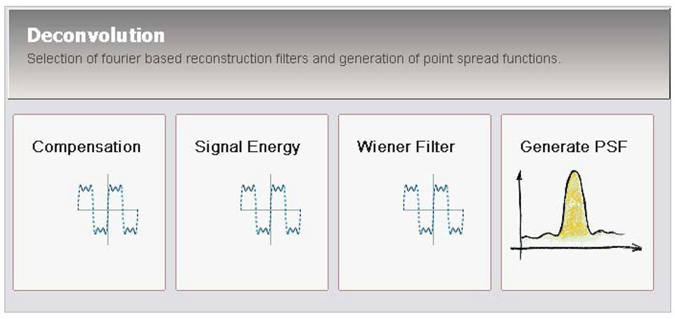
How to Carry Out Deconvolution in LCS
The resolution of two- or three-dimensional data sets is always worse than the real spatial distribution of fluorescently labeled structures. Spatial information is lost by the optical system, characterised by the point spread function (PSF). The PSF is the image of an infinitely small bright spot in the sample. If it is known, using a mathematical operation, the deconvolution, the deterioration of the resolution can be undone partially and the original structure of the object under investigation can be reconstructed partially. Resolution and contrast are enhanced. In addition, the filters implemented in the deconvolution tool in LCS (Compensation, Signal Energy, Wiener Filter) lead to a simultaneous denoising of the image. For confocal images it is only useful to apply a deconvolution procedure if the data were recorded with sufficient oversampling, i.e., the voxel size should be two or three times smaller than the resolution for the given objective lens. The resolution values can be found in the list of objectives, accessible via “Tools > Objective…” in the main menu bar.Calculation of the PSF
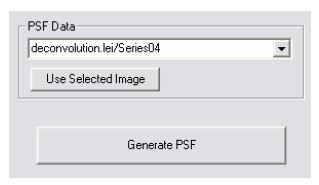
The first step is the calculation of the PSF. Clicking on the button “Generate PSF” in the path “Process > Image Processing > Enhancement > Deconvolution”:
or in the dialog windos of all three deconvolution filters:
opens another dialog window:
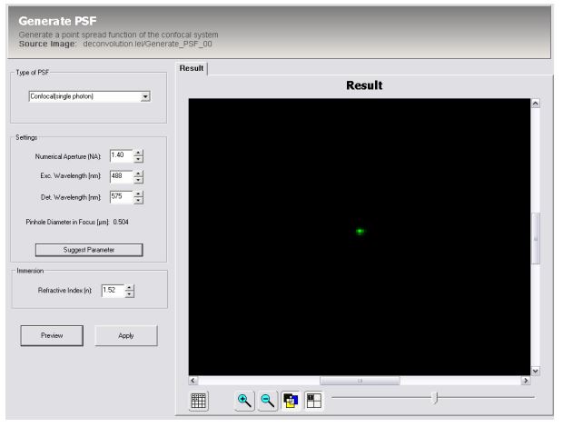
In this window, the parameters necessary for the calculation of the PSF can be set: system
type, NA of the objective lens, excitation wavelength, central wavelength of detection
window, pinhole diameter, and refractive index of the immersion medium. When clicking on
“Suggest Parameter” the parameters of the currently selected image or series (the source) are
set into the fields (as far as available).
Click on “Preview” or “Apply” to calculate a preview or a data set containing the intensity
distribution of the PSF, respectively. This data set has the same format as the source data set.
The calculation of the PSF is only possible for one-channel source data. The calculation may
take a few minutes and is under process as long as the dialog elements are disabled/grey.
Typically, in the PSF data set, non-zero intensity values are only found on a few pixels around
the center.
Filtering and deconvolution
The deconvolution filters contain an inversion of the PSF on the one hand and a noise
reduction on the other hand. The differ in the way noise is reduced.
All filters
- Select the data set containing the calculated PSF in the field “PSF Data”. With “Use
Selected Image” the data set currently selected in the “Experiment Overview” window
is selected as PSF data. - If the PSF data does not yet exist click on “Generate PSF” to calculate a PSF data set.
- Select the source data set by double-clicking on the desired file in the “Experiment
Overview” window.
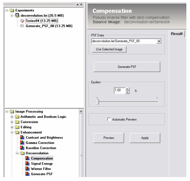
Compensation
(Also known as “Pseudoinverse filter with zero compensation”, especially useful for images
with a lot of background noise)
- Select an epsilon value as regularisation parameter.
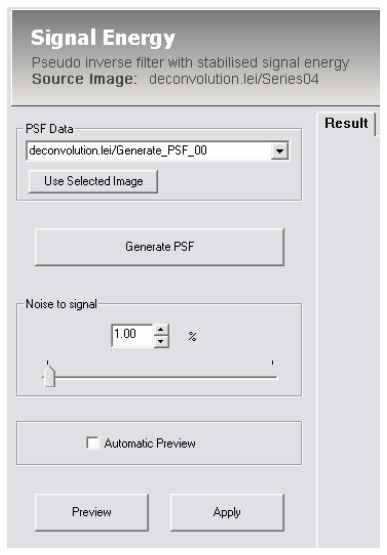
Signal Energy
(Also known as “Pseudoinverse filter with stabilised energy”)
- Select a noise-to-signal value as regularisation parameter.
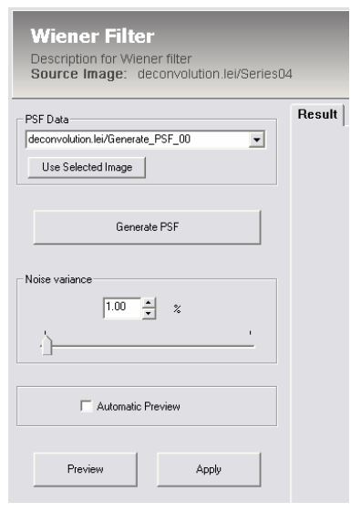
Wiener Filter
(Also known as “Pseudoinverse filter with stabilised signal energy and spectrally adapted zero
compensation”, especially useful for images with well-defined structures)
- Selecte a noise variance value as regularisation parameter.
All filters
- Click on “Preview” or “Apply” to calculate a preview or a data set containing the
deconvolved and noise-reduced data, respectively. This data set has the same format
as the source data set. - The best value for the respective regularisation parameter and the most appropriate
filtering method has to be tried out.